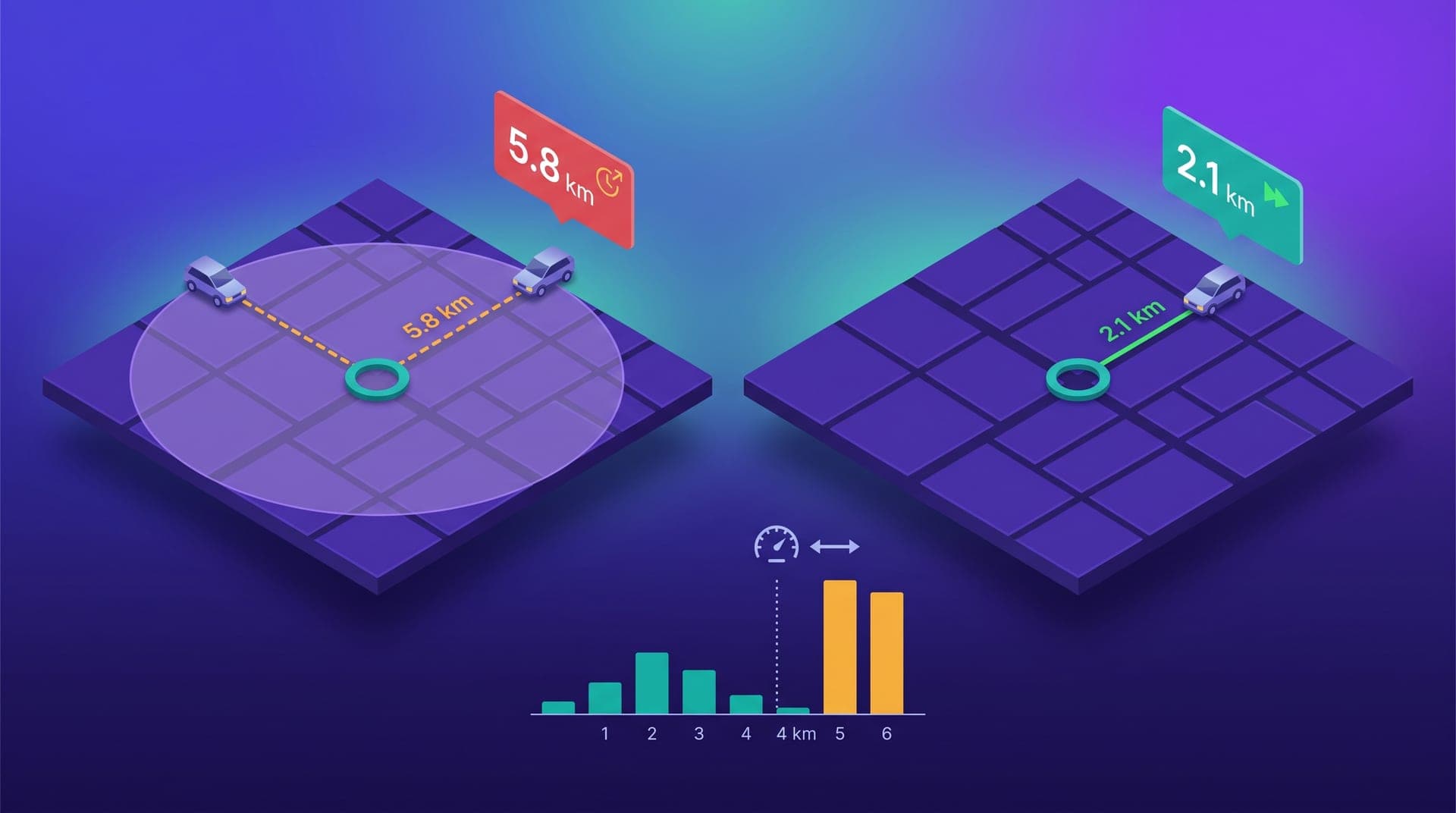
In a regional ride-hailing operation, the assignment radius — the maximum distance within which the system offers a request to an available driver — is the configuration parameter with the greatest simultaneous impact on driver rejection rate, passenger wait time, and pre-pickup cancellations. In operations with 30 to 100 weekly active drivers, most operators set this radius once at launch — typically between 4 and 8 kilometers — and don't revisit it unless a visible problem surfaces. The core issue is that a single global radius produces radically different outcomes depending on the zone: in a dense city center, driver availability keeps actual pickup distances at 1.5 to 2 kilometers even when the parameter allows 6; in a peripheral zone with the same setting and low driver density, the system assigns at 5 or 6 kilometers because no closer driver exists. Pickup distance is not merely a byproduct of fleet positioning — it is a design variable the operator can calibrate by zone and time slot to find the right balance between assignment coverage and service quality.

This article is for operators with 20 to 100 weekly active drivers who see rejection rates or wait times that vary significantly across zones but cannot diagnose whether the root cause is driver density or assignment radius configuration. It covers why pickup distance simultaneously connects the three most important operational metrics, what distance ranges drivers accept without friction depending on market type, how to query the current pickup distance distribution with the agent, how to calibrate the radius by zone without increasing requests with no available driver, how to adjust the radius by time slot when driver density shifts across the day, and what signals indicate the current radius is degrading the operation without the problem being visible in aggregate metrics. The counterintuitive thesis: reducing the first-offer radius in high-density zones improves all three metrics simultaneously, because the problem is not coverage but the distance at which the system is assigning requests that drivers are going to reject.

Why pickup distance connects all three operational metrics simultaneously

To understand why pickup distance is the central operational design variable, it helps to trace the consequence chain from a single request assigned to a driver 11 minutes away. First: a driver 11 minutes from the pickup has three times the probability of rejecting the request compared to one 4 minutes away. The unpaid 11-minute reposition — equivalent to a full short trip without income — doesn't justify the 10 to 14-minute average trip that follows in regional markets. If the driver accepts, the passenger sees an estimated arrival of 11 to 14 minutes. A passenger who sees a driver more than 10 minutes away has a cancellation rate 3 to 4 times higher than one who sees 3 to 5 minutes: the estimated wait is long enough to consider an alternative. If the passenger doesn't cancel and the trip completes, the driver arrived after consuming time and fuel without billing, reducing their effective hourly session income and making them more prone to rejecting the next long-pickup request. All three metrics — rejection, wait time, and cancellation — share a single root cause in this scenario: the pickup distance was excessive for the value of the trip. The variable connecting all three effects is not driver motivation or passenger patience: it is the distance to the pickup point at the moment of assignment.

Pickup distances drivers accept without friction: ranges by market type

Not every pickup distance triggers rejection. The driver acceptance rate as a function of distance follows a consistent pattern in regional markets across Mexico and Central America with 25 to 100 weekly active drivers. For requests less than 4 minutes away — approximately 1.5 to 2.5 kilometers in normal urban traffic — the acceptance rate is between 88 and 95%: the driver can reach the pickup and return to the next trip in a cycle compatible with their work session. Between 4 and 7 minutes — 2.5 to 4.5 kilometers — the rate drops to 72 to 82%: the reposition has a noticeable opportunity cost but the average trip compensates if the destination works for the driver. Above 7 to 8 minutes — 4.5 kilometers or more — acceptance falls below 65%: for a driver in an active session, the unpaid reposition time exceeds the threshold where most available trips justify it. These thresholds are not fixed: in markets where the average trip is under 10 minutes — short trips in compact cities of 150,000 to 250,000 residents — rejection begins earlier because the reposition-to-trip ratio deteriorates faster. In markets with average trips of 15 to 20 minutes, drivers tolerate more pickup distance because the trip income better compensates the prior reposition.

How to calculate the current pickup distance distribution

The agent query that produces the current pickup distance diagnostic: 'For the last 28 days, show me the distribution of pickup distances — the distance in kilometers between the assigned driver's position and the request point at the moment of acceptance — for completed trips. Segment that distribution by origin zone and two-hour slot. For each zone-slot combination, show me the 50th, 75th, and 90th percentile of pickup distance, the driver rejection rate, and median wait time.' The result produces three simultaneous readings. If the 75th percentile pickup distance in a zone exceeds 4.5 kilometers during a specific slot, the assignment radius is offering requests to drivers who are systematically far away. If the rejection rate in that zone-slot is above 18%, there is a direct correlation between excessive distance and rejection that confirms the diagnosis. If median wait time exceeds 8 minutes in the same combination, the reposition time of drivers who did accept is representing the dominant portion of total wait — not the distance from the acceptance point, but the cost of the long assignments that survived the rejection filter.

The 75th percentile is the reference metric because the average pickup distance can be misleading in zones with asymmetric distributions. In a zone where 70% of pickups are at 2 kilometers or less but there is a tail of long assignments at 6 or 7 kilometers, the average may sit at 3.2 kilometers — apparently acceptable — while the 75th percentile is at 4.8. That 25% of long assignments produces a disproportionate fraction of rejections and elevated wait times. What confirms the 75th percentile as the correct diagnostic indicator is that rejected requests — which don't appear in the completed pickup distance distribution because they didn't complete — likely had pickup distances equal to or greater than those that did complete. The distribution of completed trips is a lower bound on the real distribution of all assignments: the rejected ones had similar or worse distances.

Zone-level radius adjustment: why the same global parameter produces asymmetric results

The reason a fixed global assignment radius produces asymmetric effects is the difference in driver density across zones. In a city center with 15 active drivers across 6 square kilometers, a 5-kilometer radius always finds drivers within 2 to 3 kilometers: density naturally limits the actual pickup distance even if the radius permits much more. In a peripheral zone with 2 drivers across 12 square kilometers, the same 5-kilometer radius may find no driver at all or find one at 4.8 kilometers: the radius is used to its maximum because no closer option exists. The practical result: in the center, a wide radius doesn't create problematic pickup distances because density neutralizes it. In the periphery, it produces assignments at distances drivers systematically reject. And in intermediate zones — the most common in cities of 200,000 to 500,000 residents — the radius produces a mix: 65% of assignments fall within 3 kilometers, but 35% reach 4.5 or 6 kilometers, with the rejection rate from that second group elevating the global average without the operator being able to localize the cause in the aggregate metric.

Zone-level radius adjustment has two configurations operators need to distinguish. The first is the absolute maximum radius: the distance beyond which the system won't offer the request to any driver. If the zone has enough density that the system never reaches that maximum under normal conditions, reducing it changes nothing. If it consistently reaches the maximum — the 90th percentile of pickup distance is close to the configured maximum — reducing it only increases requests that expire without an available driver: it worsens completion without improving rejection. The second is the first-offer radius: the distance within which the system offers the request first, before expanding to more distant drivers if no acceptance comes within a set window. This configuration is the most effective in moderately dense zones because it assigns to nearby drivers first — reducing rejections — without leaving requests unserved when availability within the reduced radius is momentarily thin. Operators who don't distinguish between the two may reduce the maximum radius and increase unserved requests, when the correct adjustment was to reduce the first-offer radius and keep the maximum as a fallback.

Time-slot radius adjustment: why the same zone needs different settings at 7:00 and 14:00

Driver density in a zone is not constant across the day: it varies with time slot, day of week, and driver session start and end patterns. In a business district with high demand between 7:30 and 9:00 a.m., active driver density may be 0.9 drivers per square kilometer. At 2:30 p.m. in the same zone, it can drop to 0.2 drivers per square kilometer. An assignment radius that produces a median pickup distance of 2.3 kilometers during the morning peak may produce one of 5.5 kilometers during the afternoon valley with the same configuration, simply because there are four times fewer available drivers for the same area. If the operator doesn't adjust the radius by time slot, pickup distance — and with it rejections — varies dramatically without any parameter changing. That variation appears in the data as a metric degradation in certain slots without an apparent cause: the cause is that the radius configures a fixed maximum while the actual distance it produces depends on how many drivers are available within that radius at each moment.

The agent query to diagnose this variation: 'For the last 21 days, show me the median pickup distance and rejection rate for the northern zone, segmented by two-hour slot. For each slot, include the count of unique drivers who had at least one assignment in that zone during that slot.' The result shows whether the slots with the highest rejection rate coincide with the slots where driver density is lowest and median pickup distance is highest. If there is a clear correlation — the two or three highest-rejection slots are exactly the lowest-density, highest-pickup-distance ones — the intervention is adjusting the first-offer radius in that zone during those slots. The goal is not to force the system to assign farther: it is to limit the first-offer radius so the system waits for a closer driver to become available in the following seconds before expanding the search. In zones with 0.2 drivers per km² during certain hours, that adjustment produces marginally longer assignment times but substantially shorter pickup distances when drivers are available even at 3 or 4 kilometers.

How to implement the radius change without degrading coverage

The most common mistake when reducing the assignment radius is doing it without verifying that driver density within the reduced radius is sufficient to serve the zone's requests without expiration. If the zone has 1.5 available drivers per square kilometer during the adjustment slot, reducing the radius from 6 to 3 kilometers shrinks the search area by a factor of 4 — from 113 km² to 28 km² — and can leave requests unserved if those 1.5 drivers per km² aren't distributed uniformly within the reduced radius. The pre-change verification is concrete: how many unique drivers were active within the reduced radius over the previous four weeks in that zone-slot. If there are on average 3 or more drivers within 3.5 kilometers during that slot, the reduced radius has supply backing. If there are 0.8, the reduced radius will increase requests expiring without a driver before the rejection rate improves.

The assignment radius is the configuration parameter that most affects all three operational metrics simultaneously without the operator explicitly linking it to any of them in the standard dashboard. The operator who analyzes the pickup distance distribution by zone and time slot — with the 75th percentile as the diagnostic reference — has the information to determine whether the current radius is producing assignments drivers are going to reject, wait times dominated by long repositioning, or passenger cancellations caused by an excessive arrival estimate. That information transforms the radius from a technical parameter configured once at launch into an operational calibration tool the operator can adjust by zone, time slot, and season.

Pickup distance is not a problem solved by adding more drivers or improving incentives. It is a design problem solved with the right data — how far the driver travels before reaching the passenger, in which zones, and in which time slots — and with the deliberate radius adjustment that data indicates. The operator who monitors the 75th percentile pickup distance weekly, identifies the zone-slot combinations where it systematically exceeds 4.5 kilometers, and adjusts the first-offer radius in those combinations with prior availability verification gains access to simultaneous improvement in rejection, wait time, and cancellation without changing the fare or adding drivers. It is the same operation with the same resources, but with the assignment system configured to do what fleet density and geographic distribution allow: assign to drivers who are where the trip makes sense, not to those who are simply online.