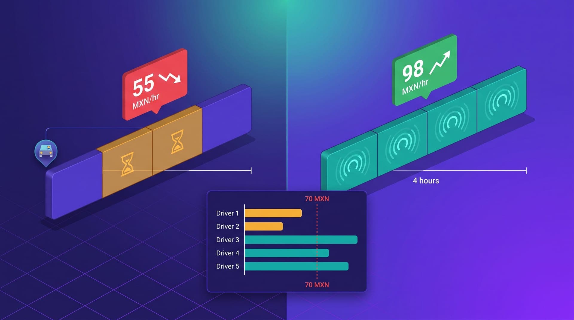
The most common metric ride-hailing operators use to assess fleet health is the number of drivers active during the week. That reading has a structural flaw: a driver who logs in for 30 minutes and completes one trip counts the same as one who works 5 continuous hours and does twelve trips. The difference between them is not in the active driver count — it is in income per active hour, the ratio of what the driver billed to the real time they dedicated to working the platform that day. When a driver who typically earns 110 MXN per active hour drops to 65 MXN over two consecutive weeks — because they spend 90 minutes of their 4-hour session waiting for requests in a zone with low demand during that time slot — they don't quit immediately: they first shorten the session, then connect fewer days, then stop appearing. The operator who only tracks total active drivers detects that process in the third or fourth week, when the driver has already decided the platform isn't worth their time.

This article is for operators with 20 to 80 active drivers who see weekly fluctuations in their available fleet without being able to identify the cause. It covers how to calculate income per active hour in a way that is comparable across drivers and weeks, what ranges signal a healthy fleet versus drivers at risk of reducing their commitment, what behavioral pattern precedes departure and how it appears in the data three to four weeks before the driver stops connecting, how off-peak positioning is the factor most affecting hourly income without changing the fare, which agent queries produce weekly tracking of this metric, and how to intervene when a driver enters the risk zone before the departure becomes irreversible. The thesis is counterintuitive for anyone who assumes churn is detected when the driver stops appearing: the data that precedes departure is visible two to three weeks earlier, in hourly income and session patterns. That window is enough to act.

The idle hour: how time without requests destroys the driver's hourly income

Income per active hour doesn't fall because the fare is low or because the driver makes shorter trips — it falls because a fraction of the driver's session time passes without requests, without revenue, and with a real opportunity cost. A driver who works from 7:00 to 11:00 a.m. in a city of 280,000 residents has four hours of available session time. If demand concentrates between 7:30 and 9:00 a.m. — the morning peak — and between 10:30 and 11:00 a.m. — the start of the midday peak — the 9:00 to 10:30 window is wait time where the driver is connected but not receiving requests at a rate that justifies their presence. If in those 90 minutes they receive two short trips producing 80 MXN and spend the rest waiting, their income for that 90-minute block is 80 MXN: equivalent to 53 MXN per hour, below the profitability threshold for most platform drivers in regional markets where the opportunity cost of one hour of work exceeds 70 MXN.

The specific problem is not that off-peak slots exist — they do in every market between the peaks — but that the driver during those slots stays in the same zone they used during the peak, where request density has already dropped. The 7:30 to 9:00 a.m. peak concentrated requests in the office zone. By 9:15, that zone has a request rate four times lower than forty minutes ago. The driver who receives no repositioning instruction at the end of the peak remains in the lowest-residual-demand zone and experiences exactly the request drought that produces low hourly income. The difference between the driver who during transition slots moves toward a zone with midday residual demand and the one who stays stationary is not in the fare or in the number of available trips: it is in the income that idle hour produces. That difference, repeated two or three times a week over four weeks, is enough for the driver to mentally reclassify the platform as a secondary option.

How to calculate income per active hour: the correct denominator

The most common error when trying to calculate income per driver hour is using total connected time as the denominator. A driver who logs in at 7:00 a.m. and disconnects at 1:00 p.m. was online for six hours, but if their first acceptance was at 7:22 and their last trip ended at 12:38, their real active time was five hours and sixteen minutes. Including the 44 minutes of connection without activity at the start and end artificially inflates the denominator and reduces the calculated hourly income, making the number appear lower than the driver's actual experience. The correct denominator is the time between the first request acceptance and the last trip completion of each session for that driver. That interval captures exactly the time the driver experienced as their active working shift and produces a metric that is comparable across drivers with different connection patterns.

The agent query that produces this metric for the past week: 'For the last 7 days, and for each driver who had at least 3 active sessions, calculate the daily income per active hour — using as the denominator the time between the first acceptance and the last trip completion of each session. Group the result by driver and show me the weekly average income per active hour, total active hours in the period, total billed, and week-over-week change for drivers with two or more weeks of history.' That result orders the fleet by income per active hour from highest to lowest and makes visible, without additional inference, which drivers have hourly income below the operational threshold. The following week, the same query referencing the prior week shows which drivers dropped and by how many points.

Operational ranges: when the number signals a driver at churn risk

In operations with 20 to 80 active drivers in cities of 150,000 to 500,000 residents in Mexico and Central America, income per active hour for drivers with more than four weeks of platform history distributes across three ranges with distinct behaviors. The healthy range is between 85 and 140 MXN per active hour: drivers in this range have sessions of 4 to 7 hours, maintain stable availability of 4 to 6 days per week, and their rejection rate is below 15%. The attention range is between 65 and 84 MXN per hour: drivers here remain active but reduce their average session by 45 to 90 minutes compared to the prior month and connect 0.5 to 1 fewer day per week. The risk range is below 65 MXN per active hour: in that range, the departure pattern — shorter sessions, fewer days connected, increasing rejection rate — manifests consistently within the following three weeks for most drivers if there is no intervention. The variation across cities is 10 to 15 MXN depending on local cost of living and fuel cost, but the behavioral thresholds are consistent.

The 65 to 70 MXN per active hour threshold is not arbitrary: it corresponds to the income level at which a platform driver using the vehicle as a work tool — with fuel costs of 4 to 7 MXN per kilometer in mid-sized cities — starts to calculate whether platform time compensates compared to other available income sources. A driver earning 65 MXN per net-of-fuel active hour obtains between 40 and 50 MXN per actual work hour: at that level, comparison with alternative activities — cargo loading, courier services, local commerce work — becomes relevant. The driver doesn't consciously run that comparison every week, but they do gradually adjust their behavior: first leaving 45 minutes before the end of their usual session, then connecting on Tuesday instead of Monday, then starting to connect only during the peaks where they know hourly income will be higher. That adjustment pattern is the precursor to departure, and it appears in the data three to four weeks before the driver stops connecting.

The pre-departure pattern: how it looks in the data before the driver leaves

What makes this pattern diagnostically useful is that each signal is measurable with data already available in the platform. Session duration and days connected per week are direct activity data. Rejection rate is already part of most operators' standard monitoring. The novelty of the hourly income diagnosis is that it connects those three metrics through a common cause: when the driver consistently experiences low hourly income for two weeks, all three indicators move simultaneously. The rejection rate rises because the driver becomes more selective, session duration falls because the driver cuts the shift during the lowest-productivity slots, and connected days drop because the driver rationalizes when it is worth connecting. The operator who tracks those three indicators per driver weekly without linking them to hourly income can see the pattern but cannot diagnose the cause or act on it.

How between-peak positioning recovers hourly income without changing the fare

The most direct intervention on driver hourly income doesn't require changing the fare or designing an additional incentive: it requires reducing dead time within the session by repositioning the driver toward zones with the highest residual request density between the main peaks. The morning peak in a city of 280,000 residents typically ends between 9:00 and 9:30 a.m. Between 9:30 and noon there is residual demand that is not a peak but does exist: health center transfers, commercial movements, mid-morning errands. That residual demand concentrates in two or three identifiable zones — the shopping area, clinics, and the market — which are not the same zones where workday peak demand was concentrated. The driver who stays in the office zone between 9:30 and 11:00 a.m. experiences the request drought that produces low hourly income. The driver who receives a repositioning instruction toward the clinic and market zone at 9:25 a.m. has requests within the next 12 to 18 minutes.

The agent query to build the residual demand map between peaks: 'For the last 21 days, show me unique requests between 9:00 a.m. and noon on Monday through Thursday, grouped by origin zone and 90-minute slot. For each zone-slot combination, show me the average daily requests and completion rate. Identify the two zones with the highest request volume in each 90-minute slot.' The result produces the between-peak residual demand map the operator can use to generate repositioning instructions at the end of the morning peak: where to go, during which slot, and what level of requests the driver can expect. For the full fleet, that transition instruction reduces idle time between peaks from 60 to 90 minutes down to 15 to 25 minutes and improves the hourly income of the set of drivers who follow it. The improvement doesn't require more drivers or more demand: it requires that available drivers be in the zones where residual demand already exists but where they aren't when the peak ends.

What to ask the agent to detect at-risk drivers before they stop connecting

The weekly query that produces the at-risk driver list: 'For the last 14 days, show me for each driver with at least 3 active sessions: income per active hour last week, income per active hour the prior week, change in days connected between weeks, and change in average session duration. Flag in red drivers who meet at least two of these conditions: income per active hour below 70 MXN last week, hourly income decline greater than 15% versus the prior week, reduction in days connected of two or more days, session duration reduction of more than one hour.' That query produces a fleet health dashboard without additional metrics: drivers flagged in red are those in the pre-departure pattern who respond to a positioning or direct communication intervention.

The intervention for at-risk drivers has two components. The first is operational: review the slots during which that driver has the most idle time — the between-peak hours where their hourly income falls below the threshold — and send them specific repositioning instructions toward zones with residual demand in those slots. The information the driver needs is the same as for proactive peak positioning: a concrete geographic reference, the time window, the expected request volume, and a reference economic data point. The second component is a direct communication: 'This week your hourly income was 62 MXN, below your usual average of 91 MXN. In the 9:30 to 11:00 a.m. slots last week there were 8 requests in the central market zone that went unserved. This week I will alert you when they start so you can move early.' That communication turns an operator data point into information the driver can use directly and signals that the operator is paying attention to their individual productivity, not just to the operation as a whole.

The operational cycle described in this series — completion rate to measure what fraction of demand is captured, assignment radius to calibrate the distance the system demands from the driver, proactive positioning to reach demand before the peak — has a sustainability prerequisite that none of those instruments measures directly: that the driver fleet stays active long enough for the operation's improvements to take hold. Income per active hour is the indicator that closes that cycle. An operation with good completion, good radius, and good positioning that loses 20% of its active fleet every month because drivers don't earn enough per hour restarts the improvement cycle from scratch with new drivers every six weeks. The operator who tracks hourly income as a fleet health metric has the information needed to prevent that restart.

The cost of not tracking driver hourly income is a number that doesn't appear in the standard dashboard. It appears in the onboarding cost of drivers who left the platform — between 200 and 400 MXN per driver in advertising, document verification time, and the initial low-productivity period — in the reduced coverage during weeks when the fleet is below its usual level, and in the lower completion rate those weeks produce. The operator who brings back the at-risk driver with concrete information — here is where they are losing a productive income hour, here is the zone where they can recover it — invests 10 minutes of agent query and a direct message to avoid the cost of a driver who doesn't return. The income the driver doesn't generate in the idle hour is the easiest income to recover in the entire operation: the demand already exists, the driver is already connected, and the only missing bridge is knowing which direction to move.